In this lesson, you will see how to quickly calculate percentages using Excel, get acquainted with the basic formula for calculating percentages, and learn a few tricks that will make your work with interest easier. For example, the formula for calculating the percentage increase, calculating the percentage of the total, and something else.
Knowing how to work with interest can be useful in a wide variety of areas of life. This will help you estimate the amount of tips in a restaurant, calculate commissions, calculate the profitability of any enterprise and the degree of your personal interest in this enterprise. Tell me honestly, would you be delighted if you were given a promo code for a 25% discount to buy a new plasma? Sounds tempting, right ?! And how much you actually have to pay, can you calculate?
In this tutorial, we will show you a few techniques to help you calculate percentages easily with Excel, as well as introduce you to the basic formulas that are used to work with percentages. You will learn some tricks and be able to hone your skills by sorting out solutions to practical problems by percentage.
Basic knowledge of interest
Term Percent(per cent) came from Latin (per centum) and was originally translated as FROM HUNDREDS... In school, you learned that percentage is a fraction of 100 parts of a whole. The percentage is calculated by division, where the desired part is in the numerator of the fraction, and the integer is in the denominator, and then the result is multiplied by 100.
The basic formula for calculating interest looks like this:
(Part / Whole) * 100 = Percentage
Example: You had 20 apples, of which 5 you distributed to your friends. What percentage of your apples did you give away? Having made simple calculations, we get the answer:
(5/20)*100 = 25%
This is how you were taught to calculate percentage in school, and you use this formula in your daily life. Calculating percentages in Microsoft Excel is an even easier task, since many mathematical operations are performed automatically.
Unfortunately, there is no universal formula for calculating percentages for all occasions. If you ask the question: what formula for calculating percentages to use to get the desired result, then the most correct answer would be: it all depends on what result you want to get.
I want to show you some interesting formulas for working with data presented as percentages. These are, for example, the formula for calculating the percentage increase, the formula for calculating the percentage of the total amount, and some more formulas that are worth paying attention to.
The basic formula for calculating percentage in Excel
The basic formula for calculating percentages in Excel looks like this:
Part / Whole = Percentage
If you compare this formula from Excel with the usual formula for percentages from a math course, you will notice that there is no multiplication by 100 in it. When calculating the percentage in Excel, you do not need to multiply the result of division by 100, since Excel will do this automatically if for a cell given Percentage format.
Now let's see how calculating percentages in Excel can help in real-world work with data. Suppose you have a certain number of ordered products (Ordered) in column B, and data on the number of delivered products (Delivered) is entered in column C. To calculate what proportion of orders have already been delivered, we will do the following:
- Write down the formula = C2 / B2 in cell D2 and copy it down as many lines as necessary using the autocomplete marker.
- Press command Percent Style(Percentage format) to display the division results in percentage format. It's on the tab Home(Home) in the group of teams Number(Number).
- If necessary, adjust the number of displayed digits to the right of the decimal point.
- Ready!
If you use any other formula to calculate percentages in Excel, the general sequence of steps remains the same.
In our example, column D contains values that show, as a percentage, what proportion of the total number of orders are already delivered orders. All values are rounded to whole numbers.
Calculating the percentage of the total in Excel
In fact, the example given is a special case of calculating the percentage of the total amount. To better understand this topic, let's look at a few more tasks. You will see how you can quickly calculate the percentage of the total in Excel using different datasets as an example.
Example 1. The total amount is calculated at the bottom of the table in a specific cell
Very often, at the end of a large data table, there is a cell labeled Total, in which the total is calculated. At the same time, we are faced with the task of calculating the share of each part relative to the total amount. In this case, the formula for calculating the percentage will look the same as in the previous example, with one difference - the cell reference in the denominator of the fraction will be absolute (with $ signs in front of the row name and column name).
For example, if you have written down some values in column B, and their total is in cell B10, then the formula for calculating percentages will be as follows:
Prompt: There are two ways to make the cell reference in the denominator absolute: either enter the sign $ manually, or select the required cell reference in the formula bar and press F4.
The figure below shows the result of calculating the percentage of the total. Percentage format with two decimal places is selected for data display.

Example 2. Parts of the total amount are on multiple lines
Imagine a table with data like the previous example, but here the product data is scattered across multiple rows in the table. It is required to calculate what part of the total amount is made up of orders for a specific product.
In this case, we use the function SUMIF(SUMIF). This function allows you to sum up only those values that meet a certain criterion, in our case, this is a given product. We use this result to calculate the percentage of the total.
SUMIF (range, criteria, sum_range) / total
= SUMIF (range, criterion, sum_range) / total
In our example, column A contains the names of products (Product) - this is range... Column B contains data about the quantity (Ordered) - this is sum_range... In cell E1 we enter our criterion- the name of the product for which you want to calculate the percentage. The total for all products is calculated in cell B10. The working formula will look like this:
SUMIF (A2: A9, E1, B2: B9) / $ B $ 10
= SUMIF (A2: A9, E1, B2: B9) / $ B $ 10

By the way, the name of the product can be entered directly into the formula:
SUMIF (A2: A9, "cherries", B2: B9) / $ B $ 10
= SUMIF (A2: A9; "cherries"; B2: B9) / $ B $ 10
If you need to calculate how much of the total amount is made up of several different products, you can add up the results for each of them and then divide by the total amount. For example, this is how the formula will look if we want to calculate the result for cherries and apples:
= (SUMIF (A2: A9, "cherries", B2: B9) + SUMIF (A2: A9, "apples", B2: B9)) / $ B $ 10
= (SUMIF (A2: A9; "cherries"; B2: B9) + SUMIF (A2: A9; "apples"; B2: B9)) / $ B $ 10
How to calculate percentage change in Excel
One of the most popular tasks that you can accomplish with Excel is calculating percent change in data.
Excel formula that calculates percentage change (increase / decrease)
(B-A) / A = Percentage change
Using this formula in working with real data, it is very important to correctly determine what value to put in place. A, and which one - in place B.
Example: Yesterday you had 80 apples, and today you have 100 apples. This means that today you have 20 more apples than yesterday, that is, your result is an increase of 25%. If yesterday there were 100 apples, and today there are 80 - then this is a 20% decrease.
So, our formula in Excel will work as follows:
(New value - Old value) / Old value = Change in percentage
Now let's see how this formula works in Excel in practice.
Example 1. Calculating the percentage change between two columns
Suppose that column B contains the prices for the last month (Last month), and column C contains the prices that are current for this month (This month). Let's enter the following formula in column D to calculate the price change from the last month to the current one as a percentage.
This formula calculates the percentage change (increase or decrease) in the price this month (column C) compared to the previous month (column B).
After you write the formula in the first cell and copy it to all the necessary lines by pulling the autocomplete marker, do not forget to set Percentage format for cells with formula. As a result, you should have a table similar to the one shown in the figure below. In our example, positive data, which shows an increase, are displayed in standard black, and negative values (decrease in percentage) are highlighted in red. For details on how to set up such formatting, read this article.

Example 2. Calculating the percentage change between lines
In the case when your data is located in one column, which reflects information about sales per week or per month, the change in percentage can be calculated using the following formula:
Here C2 is the first value and C3 is the next value in order.
Comment: Please note that with such an arrangement of data in the table, the first row with the data must be skipped and the formula must be written from the second row. In our example, this will be cell D3.
After you write down the formula and copy it into all the necessary rows of your table, you should get something similar to this:

For example, this is how the formula for calculating the percentage change for each month in comparison with the indicator will look like January(January):
When you copy your formula from one cell to all the others, the absolute reference will remain unchanged, while the relative reference (C3) will change to C4, C5, C6, and so on.

Calculating the value and total amount based on a known percentage
As you can see, calculating percentages in Excel is easy! It is just as easy to calculate the value and the total amount at a known percentage.
Example 1. Calculating a value based on a known percentage and total amount
Suppose you buy a new computer for $ 950, but to this price you need to add 11% VAT. The question is - how much do you need to pay extra? In other words, 11% of the indicated cost is how much in foreign currency?
This formula will help us:
Total * Percentage = Amount
Total Amount * Interest = Value
Let's pretend that total amount(Total) is written in cell A2, and Interest(Percent) - in cell B2. In this case, our formula will look pretty simple = A2 * B2 and will give the result $104.50 :

It is important to remember: When you manually enter a numeric value in a table cell and after it a% sign, Excel understands this as hundredths of the entered number. That is, if you enter 11% from the keyboard, then in fact the value 0.11 will be stored in the cell - this is the value Excel will use when performing calculations.
In other words, the formula = A2 * 11% is equivalent to the formula = A2 * 0.11... Those. in formulas, you can use either decimal values or values with a percent sign - whichever is more convenient for you.
Example 2. Calculation of the total amount based on a known percentage and value
Let's say your friend offered to buy his old computer for $ 400 and said it was 30% cheaper than its full price. Do you want to know how much this computer originally cost?
Since 30% is a decrease in the price, the first thing we do is subtract this value from 100% in order to calculate how much of the original price you need to pay:
Now we need a formula that will calculate the initial price, that is, find the number, 70% of which is equal to $ 400. The formula will look like this:
Amount / Percentage = Total
Value / Percentage = Total
To solve our problem, we will receive the following form:
A2 / B2 or = A2 / 0.7 or = A2 / 70%

How to increase / decrease a value by a percentage
With the onset of the holiday season, you will notice certain changes in your usual weekly items of expenditure. You may want to make some additional adjustments to the calculation of your spending limits.
To increase the value by a percentage, use the following formula:
Value * (1 +%)
For example, the formula = A1 * (1 + 20%) takes the value in cell A1 and increases it by 20%.
To decrease the value by a percentage, use the following formula:
Value * (1-%)
For example, the formula = A1 * (1-20%) takes the value in cell A1 and decreases it by 20%.
In our example, if A2 is your current expenses, and B2 is the percentage by which you want to increase or decrease their value, then you need to write the following formula in cell C2:
Increase by percentage: = A2 * (1 + B2)
Decrease by percentage: = A2 * (1-B2)

How to increase / decrease all values in a column by a percentage
Suppose you have a whole column filled with data that needs to be increased or decreased by some percentage. In this case, you do not want to create another column with the formula and new data, but change the values in the same column.
We need only 5 steps to solve this problem:

In both formulas, we took 20% as an example, and you can use the percentage value that you need.

As a result, the values in column B will increase by 20%.

In this way, you can multiply, divide, add or subtract a percentage from a whole column of data. Just enter the percentage you want in the blank cell and follow the steps outlined above.
These methods will help you calculate percentages in Excel. And even if percent has never been your favorite area of mathematics, knowing these formulas and techniques, you will make Excel do all the work for you.
That's all for today, thank you for your attention!
Interest is everywhere in the world today. Not a day goes by without using them. Buying products - we pay VAT. Taking a loan from the bank, we pay the amount with interest. When we compare income, we also use interest.
Working with percentages in Excel
Before starting work in Microsoft Excel, let's remember school math lessons, where you studied fractions and percentages.
When working with percentages, remember that one percent is one hundredth (1% = 0.01).
Performing the action of adding percent (for example, 40 + 10%), first we find 10% of 40, and only then we add the base (40).
When working with fractions, do not forget about the basic rules of mathematics:
- Multiplying by 0.5 is equal to dividing by 2.
- Any percentage is expressed as a fraction (25% = 1/4; 50% = 1/2, etc.).
We count the percentage of the number
To find the percentage of a whole number, divide the desired fraction by an integer and multiply the result by 100.
Example # 1. The warehouse contains 45 units of goods. 9 units of the product were sold in a day. How much was sold as a percentage?
9 is a part, 45 is a whole. We substitute the data into the formula:
(9/45)*100=20%
We do the following in the program:
How did it come about? Having set the percentage type of calculations, the program will independently add the formula for you and put a "%" sign. If we set the formula ourselves (multiplied by one hundred), then the "%" sign would not exist!
Example No. 2. Let's solve the inverse problem. It is known that there are 45 units of goods in the warehouse. It is also indicated that only 20% were sold. How many units were sold in total?
Example No. 3... Let's try the acquired knowledge in practice. We know the price for the product (see the picture below) and VAT (18%). You want to find the amount of VAT.
We multiply the price of the product by the percentage, according to the formula B1 * 18%. 
Advice! Do not forget to extend this formula to the rest of the lines. To do this, grab the lower right corner of the cell and lower it to the end. Thus, we get an answer to several elementary problems at once.

Example No. 4. Inverse problem. We know the amount of VAT for the product and the rate (18%). You want to find the price of an item.

Add and subtract
Let's start by adding... Let's consider the problem with a simple example:
- We are given the price of the item. It is necessary to add to it the VAT percentage (VAT is 18%).

- If we use the formula B1 + 18%, then we get the wrong result. This is because we need to add not just 18%, but 18% of the first amount. As a result, we get the formula B1 + B1 * 0.18 or B1 + B1 * 18%.

- Pull down to get all answers at once.

- In case you use the formula B1 + 18 (without the% sign), then the answers will be obtained with "%" signs, and the results are not what we need.

- But this formula will also work if we change the cell format from "percentage" to "number".

- You can remove the number of decimal places (0) or set it at your discretion.

Now let's try to subtract the percentage from the number... With the knowledge of addition, subtraction will not be difficult. Everything will work by replacing one sign "+" with "-". The working formula will look like this: B1-B1 * 18% or B1-B1 * 0.18. 
Now we will find percentage of all sales. To do this, let's sum up the quantity of goods sold and use the formula B2 / $ B $ 7.
These are the basic tasks. It seems simple, but many people make mistakes.
Making a percentage chart
There are several types of charts. Let's consider them separately.
Pie chart
Let's try to create a pie chart. It will display the percentage of products sold. First, we are looking for a percentage of all sales.
Schedule
Instead of a histogram, you can use a graph. For example, the histogram is not suitable for tracking profit. It would be more appropriate to use a graph. The graph is inserted in the same way as the histogram. It is necessary to select a chart in the "Insert" tab. One more chart can be superimposed on this chart. For example, a chart with losses. 
This is where we end. Now you know how to rationally use percentages, build charts and graphs in Microsoft Excel. If you have a question that the article did not answer,. We will try to help you.
Microsoft Office Excel spreadsheet editor is often overlooked in vain. It seems to many that it is difficult to understand, so they use a calculator and other available tools to solve their problems. But why do this, if with the help of this editor you can simply recalculate formulas in batches, build graphs, tables almost completely automatically. And you can master the Excel database in a couple of days. If you want to explore all the functionality of this utility, then visit the site https://tutorexcel.ru/. There you can find any answer to your Excel question.Add interest
Often times, people need to add interest. To avoid doing this manually, you just need to use Excel. And we'll tell you how.Let's say that to a certain number, you need to add some kind of fixed percentage. To do this, in cell A1 we enter our amount, from which the percentage will be derived. It will appear in cell A2. But first, we do the following. As we said above, the percentage in this example is fixed. First, we determine the magnitude of the multiplier. You can't just enter 25% (our example). To do this, use the formula 1+ (25/100) = 1.25. The resulting value is our multiplier, which must be written into cell A2. To do this, click on it and enter the following: equal sign, source cell number (A1), asterisk and multiplier. It looks like this: = A1 * 1.25. Now it remains to confirm the result by pressing the Enter key. The program will give you the result in a matter of seconds.
But, it does not always happen that you need to multiply by a fixed percentage. If it changes, then you have to use three cells.
In the first, as in the previous case, we enter our number. In the second B1 we will enter our percentage. And finally, cell C1 is the result. In order to calculate the percentage, we enter the following formula in C1: A1 * (1 + B1 / 100). A1 is the original number and B1 is the percentage. In this case, we write the cell number so that when the percentage value changes, the formula does not change. She will automatically substitute the number from B1. After that, press Enter and get the finished result.
As you can see, everything is extremely simple and straightforward. MS Excel is a multifunctional editor that is quite easy to learn, but nevertheless has the best basis for working with graphs, tables and formulas.
Excel is used very often because of the simplicity of building tables. Most SEO specialists use it to group keywords for their semantic core.
Working in Excel, it is often necessary to add or subtract some percentage from the number. This may be due to the need to add VAT percentage or calculate profit. Whatever the specific task, it can be solved in Excel.
Now we are going to show you how to add a percentage to a number in Excel. The material will be useful for users of all versions of Excel, including Excel 2003, 2007, 2010, 2013 and 2016.
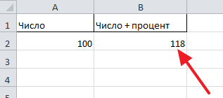
To explain how to add a percentage to a number, consider a simple example. Let's say you have a number to which you need to add a certain percentage (for example, you need to add 18% VAT). And in the next cell, you want to get the value with the already added percentage.
To do this, you need to select the cell where the result should be located and enter the formula in it. As a formula, you can use just such a simple structure: = A2 + A2 * 18%. Where A2 is the cell containing the original number, and 18 is the percentage you want to add to that original number.

After you have entered the formula, you just need to press the Enter key on your keyboard and you will get the result. In our case, we added 18 percent to 100 and got 118.
If you want not to add a percentage, but subtract it, then this is done in a similar way. Only the formula uses not a plus, but a minus.

If necessary, the percentage that you will add or subtract can not be indicated directly in the formula, but taken from the table. For this case, the formula needs to be slightly changed: = A2 + A2 * B2%. As you can see, the formula uses the cell address instead of a specific percentage value, followed by the percentage.

After using such a formula, you will receive a number with the percentage added to it, which was indicated in the table.

Potential problem with adding interest
It should be noted that when working with percentages, you may get lost in the fact that some too large numbers, as well as a percent sign, will start to appear in your cells.
This happens when the user first enters the wrong formula and then corrects it. For example, if you add 18 percent, you can make a mistake and enter: = A2 + 18%.

If after that you correct and enter the correct formula = A2 + A2 * 18%, then you will get some incredibly large number.

The problem is that as a result of the introduction of the first formula, the cell format changed from numeric to percentage. To fix this, right-click on the cell and go to "Format Cells".

In the window that opens, select the cell format that will suit her.

Most often, it is general or numeric. After selecting the required format, save the settings using the "Ok" button.
In this tutorial, you will learn various useful formulas for adding and subtracting dates in Excel. For example, you will learn how to subtract another from one date, how to add several days, months or years to a date, etc.
If you have already taken lessons on working with dates in Excel (ours or any other lessons), then you should know the formulas for calculating units of time, such as days, weeks, months, years.
When analyzing dates in any data, you often need to perform arithmetic operations on these dates. This article will explain some formulas for adding and subtracting dates that you might find helpful.
How to subtract dates in Excel
Suppose that you have in the cells A2 and B2 contains dates, and you need to subtract one date from another to find out how many days are between them. As is often the case in Excel, this result can be obtained in several ways.
Example 1. Directly subtract one date from another
I think you know that Excel stores dates as integers, starting at 1, which corresponds to January 1, 1900. Therefore, you can simply arithmetically subtract one number from the other:
Example 2. Subtracting dates using the DATEDIT function
If the previous formula seems too simple to you, you can get the same result in a more sophisticated way using the function DATEDATE(DATEDIF).
DATEDATE (A2; B2; "d")
= DATEDIF (A2, B2, "d")
The following figure shows that both formulas return the same result, except for row 4, where the function DATEDATE(DATEDIF) returns an error #NUMBER!(#NUM!). Let's see why this is happening.
When you subtract a later date (May 6, 2015) from an earlier date (May 1, 2015), the subtraction operation returns a negative number. However, the syntax of the function DATEDATE(DATEDIF) does not allow start date was more end date and naturally returns an error.
Example 3. Subtract the date from the current date
To subtract a specific date from the current date, you can use any of the previously described formulas. Just use the function instead of today's date TODAY(TODAY):
TODAY () - A2
= TODAY () - A2
DATEDATE (A2, TODAY (), "d")
= DATEDIF (A2, TODAY (), "d")
As in the previous example, the formulas work fine when the current date is greater than the date to be subtracted. Otherwise the function DATEDATE(DATEDIF) returns an error.

Example 4. Subtracting dates using the DATE function
If you prefer to enter dates directly in the formula, specify them using the function DATE(DATE) and then subtract one date from the other.
Function DATE has the following syntax: DATE( year; month; day) .
For example, the following formula subtracts May 15, 2015 from May 20, 2015 and returns a difference of 5 days.
DATE (2015; 5; 20) -DATE (2015; 5; 15)
= DATE (2015,5,20) -DATE (2015,5,15)

If needed count the number of months or years between two dates, then the function DATEDATE(DATEDIF) is the only possible solution. In the continuation of the article, you will find several examples of formulas that describe this function in detail.
Now that you know how to subtract one date from another, let's see how you can add or subtract a certain number of days, months or years from a date. There are several Excel functions for this. What exactly to choose depends on which units of time you want to add or subtract.
How to add (subtract) days to a date in Excel
If you have a date in a cell or a list of dates in a column, you can add (or subtract) a certain number of days to them using the appropriate arithmetic operation.
Example 1. Adding days to a date in Excel
The general formula for adding a certain number of days to a date looks like this:
= date + N days
The date can be set in several ways:
- By reference to the cell:
- Calling a function DATE(DATE):
DATE (2015; 5; 6) +10
= DATE (2015,5,6) +10 - Calling another function. For example, to add several days to the current date, use the function TODAY(TODAY):
TODAY () + 10
= TODAY () + 10
The following figure shows the effect of these formulas. At the time of writing, the current date is May 6, 2015.

Note: The result of these formulas is an integer representing the date. To show it as a date, you need to select a cell (or cells) and click Ctrl + 1... A dialog box will open Cell format(Format Cells). In the tab Number(Number) from the list of number formats, select date(Date) and then specify the format you want. A more detailed description can be found in the article.
Example 2. Subtracting days from a date in Excel
To subtract a specific number of days from a date, you again need to use normal arithmetic operation. The only difference from the previous example is minus instead of plus
= date - N days
Here are some examples of formulas:
A2-10
= DATE (2015; 5; 6) -10
= TODAY () - 10

How to add (subtract) several weeks to a date
When you need to add (subtract) several weeks to a certain date, you can use the same formulas as before. You just need to multiply the number of weeks by 7:
- Add N weeks to date in Excel:
A2 + N weeks * 7
For example, to add 3 weeks to the date in a cell A2, use the following formula:
- Subtract N weeks from date to Excel:
A2 - N weeks * 7
To subtract 2 weeks from today's date, use this formula:
TODAY () - 2 * 7
= TODAY () - 2 * 7
How to add (subtract) several months to a date in Excel
To add (or subtract) a certain number of months to a date, you need to use the function DATE(DATE) or DATE(EDATE) as shown below.
Example 1. Add several months to a date using the DATE function
If the list of dates is, for example, in the column A, indicate the number of months you want to add (positive number) or subtract (negative number) in some cell, say, in C2.
Enter into cell B2 the formula below, click on the selected corner of the cell and drag it down the column with the mouse B to the last filled cell in the column A... Formula from cell B2 will be copied to all cells in the column B.
DATE (YEAR (A2); MONTH (A2) + $ C $ 2; DAY (A2))
= DATE (YEAR (A2), MONTH (A2) + $ C $ 2, DAY (A2))

Let's see what this formula does. The logic of the formula is clear and obvious. Function DATE( year; month; day) receives the following arguments:
- Year from date in cell A2;
- Month from date in cell A2+ number of months in the cell C2;
- Day from date in cell A2;
It's that simple! If you enter in C2 negative number, the formula will subtract months, not add.

Naturally, nothing prevents you from entering a minus right in the formula to subtract months:
DATE (YEAR (A2); MONTH (A2) - $ C $ 2; DAY (A2))
= DATE (YEAR (A2), MONTH (A2) - $ C $ 2, DAY (A2))
And, of course, you can specify the number of months to add or subtract directly in the formula without reference to a cell. The finished formulas will look something like this:
- Add months to date:
DATE (YEAR (A2); MONTH (A2) +2; DAY (A2))
= DATE (YEAR (A2), MONTH (A2) + 2, DAY (A2)) - Subtract months from date:
DATE (YEAR (A2); MONTH (A2) -2; DAY (A2))
= DATE (YEAR (A2), MONTH (A2) -2, DAY (A2))
Example 2. Add or subtract months from a date using the EDATE function
Excel provides a special function that returns a date that is a certain number of months back or forward from a given date - this is the function DATE(EDATE). It is available in the latest versions of Excel 2007, 2010, 2013 and the new Excel 2016.
Using DATE(EDATE) You supply the following two arguments:
- Start date - the date from which the number of months is counted.
- Months - the number of months to add (positive number) or subtract (negative number).
These formulas will give the same result as formulas with the function DATE(DATE) in the previous example:

When using the function DATE(EDATE) The start date and number of months can be specified directly in the formula. Dates can be set using the function DATE(DATE) or as a result of other formulas. For example:
- This formula adds 10 months to May 7, 2015
DATE (DATE (2015; 5; 7); 10)
= EDATE (DATE (2015,5,7), 10) - This formula subtracts 10 months from today's date
DATE (TODAY (); - 10)
= EDATE (TODAY (), - 10)
Note: Function DATE(EDATE) returns just an integer. To represent it as a date, you must apply a date format to the cell. How to do this is indicated in the article. How to change date format in Excel.
How to add (subtract) years to a date in Excel
Adding years to dates in Excel is the same as adding months. You need to use the function again DATE(DATE), but this time you need to specify the number of years you want to add:
DATE (YEAR ( date) + N years; MONTH( date); DAY( date))
= DATE (YEAR ( date) + N years, MONTH ( date), DAY ( date))
On an Excel sheet, formulas might look like this:
- Add 5 years to the date specified in the cell A2:
DATE (YEAR (A2) +5; MONTH (A2); DAY (A2))
= DATE (YEAR (A2) + 5, MONTH (A2), DAY (A2)) - Subtract 5 years from the date given in the cell A2:
DATE (YEAR (A2) -5; MONTH (A2); DAY (A2))
= DATE (YEAR (A2) -5, MONTH (A2), DAY (A2))
To get a universal formula, you can enter the number of years in a cell, and then refer to that cell in the formula. A positive number will add years to the date, and a negative number will subtract it.

Add (subtract) days, months and years to a date
If you carefully read the two previous examples, then I think you have guessed how to add (or subtract) years, months and days to a date in one formula at once. Yes, using the good old function DATE(DATA)!
- For additions X years, Y months and Z days:
DATE (YEAR ( date) + X years; MONTH( date) + Y months; DAY( date) + Z days)
= DATE (YEAR ( date) + X years, MONTH ( date) + Y months, DAY ( date) + Z days) - For subtraction X years, Y months and Z days:
DATE (YEAR ( date) - X years; MONTH( date) - Y months; DAY( date) - Z days)
= DATE (YEAR ( date) - X years, MONTH ( date) - Y months, DAY ( date) - Z days)
For example, the following formula adds 2 years and 3 months, and subtracts 15 days from the date in the cell A2:
DATE (YEAR (A2) +2; MONTH (A2) +3; DAY (A2) -15)
= DATE (YEAR (A2) + 2, MONTH (A2) + 3, DAY (A2) -15)
For our date column, the formula looks like this:
DATE (YEAR (A2) + $ C $ 2; MONTH (A2) + $ D $ 2; DAY (A2) + $ E $ 2)
= DATE (YEAR (A2) + $ C $ 2, MONTH (A2) + $ D $ 2, DAY (A2) + $ E $ 2)

How to add and subtract times in Excel
In Microsoft Excel, you can add and subtract times using the function TIME(TIME). It allows you to treat time units (hours, minutes, and seconds) the same way you treat years, months, and days in a function. DATE(DATE).
- Add time in Excel:
A2 + TIME ( watch; minutes; seconds)
= A2 + TIME ( watch, minutes, seconds) - Subtract time in Excel:
A2 - TIME ( watch; minutes; seconds)
= A2 - TIME ( watch, minutes, seconds)where A2 Is a cell with a time that needs to be changed.
For example, to add 2 hours 30 minutes and 15 seconds to the time in a cell A2 you need to use the following formula:
A2 + TIME (2; 30; 15)
= A2 + TIME (2,30,15)
A2 + TIME (2; 30; -15)
= A2 + TIME (2,30, -15)
You can also enter the desired values in the cells of the worksheet and refer to them in the formula:
A2 + TIME ($ C $ 2; $ D $ 2; $ E $ 2)
= A2 + TIME ($ C $ 2, $ D $ 2, $ E $ 2)


