National Research University

Department of Applied Geology

Essay on higher mathematics

On the topic: "Basic elementary functions,

their properties and graphs"

Completed:

Checked:

teacher

Definition. The function given by the formula y=a x (where a>0, a≠1) is called an exponential function with base a.

Let us formulate the main properties of the exponential function:

1. The domain of definition is the set (R) of all real numbers.

2. The range of values ​​is the set (R+) of all positive real numbers.

3. When a > 1, the function increases on the entire real line; at 0<а<1 функция убывает.

4. Is a general function.

, on the interval xО [-3;3] , on the interval xО [-3;3]

A function of the form y(х)=х n , where n is the number ОR, is called a power function. The number n can take on different values: both integer and fractional, both even and odd. Depending on this, the power function will have a different form. Consider special cases that are power functions and reflect the main properties of this type of curves in the following order: power function y \u003d x² (a function with an even exponent - a parabola), a power function y \u003d x³ (a function with an odd exponent - a cubic parabola) and function y \u003d √ x (x to the power of ½) (function with a fractional exponent), a function with a negative integer exponent (hyperbola).

Power function y=x²

1. D(x)=R – the function is defined on the entire numerical axis;

2. E(y)= and increases on the interval

Power function y=x³

1. The graph of the function y \u003d x³ is called a cubic parabola. The power function y=x³ has the following properties:

2. D(x)=R – the function is defined on the entire numerical axis;

3. E(y)=(-∞;∞) – the function takes all values ​​in its domain of definition;

4. When x=0 y=0 – the function passes through the origin O(0;0).

5. The function increases over the entire domain of definition.

6. The function is odd (symmetric about the origin).

, on the interval xн [-3;3]

Depending on the numerical factor in front of x³, the function can be steep / flat and increase / decrease.

Power function with integer negative exponent:

If the exponent n is odd, then the graph of such a power function is called a hyperbola. A power function with a negative integer exponent has the following properties:

1. D(x)=(-∞;0)U(0;∞) for any n;

2. E(y)=(-∞;0)U(0;∞) if n is an odd number; E(y)=(0;∞) if n is an even number;

3. The function decreases over the entire domain of definition if n is an odd number; the function increases on the interval (-∞;0) and decreases on the interval (0;∞) if n is an even number.

4. The function is odd (symmetric about the origin) if n is an odd number; a function is even if n is an even number.

5. The function passes through the points (1;1) and (-1;-1) if n is an odd number and through the points (1;1) and (-1;1) if n is an even number.

, on the interval xн [-3;3]

Power function with fractional exponent

A power function with a fractional exponent of the form (picture) has a graph of the function shown in the figure. A power function with a fractional exponent has the following properties: (picture)

1. D(x) ОR, if n is an odd number and D(x)= , on the interval xО , on the interval xО [-3;3]

The logarithmic function y \u003d log a x has the following properties:

1. Domain of definition D(x)н (0; + ∞).

2. Range of values ​​E(y) О (- ∞; + ∞)

3. The function is neither even nor odd (general).

4. The function increases on the interval (0; + ∞) for a > 1, decreases on (0; + ∞) for 0< а < 1.

The graph of the function y = log a x can be obtained from the graph of the function y = a x using a symmetry transformation about the line y = x. In Figure 9, a plot of the logarithmic function for a > 1 is plotted, and in Figure 10 - for 0< a < 1.

; on the interval xн ; on the interval xО

The functions y \u003d sin x, y \u003d cos x, y \u003d tg x, y \u003d ctg x are called trigonometric functions.

The functions y \u003d sin x, y \u003d tg x, y \u003d ctg x are odd, and the function y \u003d cos x is even.

Function y \u003d sin (x).

1. Domain of definition D(x) ОR.

2. Range of values ​​E(y) О [ - 1; one].

3. The function is periodic; the main period is 2π.

4. The function is odd.

5. The function increases on the intervals [ -π/2 + 2πn; π/2 + 2πn] and decreases on the intervals [ π/2 + 2πn; 3π/2 + 2πn], n О Z.

The graph of the function y \u003d sin (x) is shown in Figure 11.

Schoolchildren are faced with the task of constructing a function graph at the very beginning of studying algebra and continue to build them from year to year. Starting from a graph of a linear function, for the construction of which you need to know only two points, to a parabola, for which you already need 6 points, a hyperbola and a sinusoid. Every year, the functions become more and more complex and it is no longer possible to plot their graphs according to a template, it is necessary to conduct more complex studies using derivatives and limits.

Let's figure out how to find the graph of a function? To do this, let's start with the simplest functions, the graphs of which are built by points, and then consider a plan for constructing more complex functions.

Plotting a Linear Function

To build the simplest graphs, a table of function values ​​is used. The graph of a linear function is a straight line. Let's try to find the points of the graph of the function y=4x+5.

1. To do this, we take two arbitrary values ​​of the variable x, substitute them one by one into the function, find the value of the variable y and put everything in the table.
2. Let's take the value x=0 and substitute it into the function instead of x - 0. We get: y=4*0+5, that is, y=5 write this value to the table under 0. Similarly, take x=0 we get y=4*1+5 , y=9.
3. Now, to build a function graph, you need to plot these points on the coordinate plane. Then you need to draw a straight line.

Plotting a Quadratic Function

A quadratic function is a function of the form y=ax 2 +bx +c, where x is a variable, a,b,c are numbers (a is not equal to 0). For example: y=x 2 , y=x 2 +5, y=(x-3) 2 , y=2x 2 +3x+5.

To build the simplest quadratic function y=x 2 usually take 5-7 points. Let's take the values ​​for the variable x: -2, -1, 0, 1, 2 and find the values ​​of y in the same way as when building the first graph.

The graph of a quadratic function is called a parabola. After constructing function graphs, students have new tasks associated with the graph.

Example 1: find the abscissa of the function graph point y=x 2 if the ordinate is 9. To solve the problem, you need to substitute its value 9 instead of y into the function. We get 9=x 2 and solve this equation. x=3 and x=-3. This can also be seen in the graph of the function.

Investigation of a function and construction of its graph

To plot more complex functions, several steps must be taken to study it. For this you need:

1. Find the scope of the function. The scope is all the values ​​that x can take on. From the domain of definition, one should exclude those points at which the denominator becomes 0 or the radical expression becomes negative.
2. Set even or odd function. Recall that even is the function that meets the condition f(-x)=f(x). Its graph is symmetrical with respect to Oy. A function will be odd if it meets the condition f(-x)=-f(x). In this case, the graph is symmetrical about the origin.
3. Find points of intersection with coordinate axes. In order to find the abscissa of the point of intersection with the x-axis, it is necessary to solve the equation f(x)=0 (the ordinate is 0). To find the ordinate of the point of intersection with the Oy axis, it is necessary to substitute 0 in the function instead of the x variable (the abscissa is 0).
4. Find the asymptotes of the function. An asymptote is a line that the graph approaches indefinitely, but never crosses. Let's figure out how to find the asymptotes of the graph of a function.
   • Vertical asymptote straight line of the form x=a
   • Horizontal asymptote - a straight line of the form y \u003d a
   • Oblique asymptote - straight line of the form y=kx+b
5. Find the extremum points of the function, the intervals of increase and decrease of the function. Find the extremum points of the function. To do this, you need to find the first derivative and equate it to 0. It is at these points that the function can change from increasing to decreasing. Let us determine the sign of the derivative on each interval. If the derivative is positive, then the graph of the function increases; if it is negative, it decreases.
6. Find the inflection points of the graph of the function, the intervals of convexity up and down.

Finding inflection points is now easier than ever. You just need to find the second derivative, then equate it to zero. Next, we find the sign of the second derivative on each interval. If positive, then the graph of the function is convex down, if negative - up.

This methodological material is for reference only and covers a wide range of topics. The article provides an overview of the graphs of the main elementary functions and considers the most important issue - how to correctly and FAST build a graph. In the course of studying higher mathematics without knowing the graphs of the basic elementary functions, it will be difficult, so it is very important to remember what the graphs of a parabola, hyperbola, sine, cosine, etc. look like, to remember some function values. We will also talk about some properties of the main functions.

I do not pretend to completeness and scientific thoroughness of the materials, the emphasis will be placed, first of all, on practice - those things with which one has to face literally at every step, in any topic of higher mathematics. Charts for dummies? You can say so.

By popular demand from readers clickable table of contents:

In addition, there is an ultra-short abstract on the topic
– master 16 types of charts by studying SIX pages!

Seriously, six, even I myself was surprised. This abstract contains improved graphics and is available for a nominal fee, a demo version can be viewed. It is convenient to print the file so that the graphs are always at hand. Thanks for supporting the project!

And we start right away:

How to build coordinate axes correctly?

In practice, tests are almost always drawn up by students in separate notebooks, lined in a cage. Why do you need checkered markings? After all, the work, in principle, can be done on A4 sheets. And the cage is necessary just for the high-quality and accurate design of the drawings.

Any drawing of a function graph starts with coordinate axes.

Drawings are two-dimensional and three-dimensional.

Let us first consider the two-dimensional case Cartesian coordinate system:

1) We draw coordinate axes. The axis is called x-axis , and the axis y-axis . We always try to draw them neat and not crooked. The arrows should also not resemble Papa Carlo's beard.

2) We sign the axes with capital letters "x" and "y". Don't forget to sign the axes.

3) Set the scale along the axes: draw zero and two ones. When making a drawing, the most convenient and common scale is: 1 unit = 2 cells (drawing on the left) - stick to it if possible. However, from time to time it happens that the drawing does not fit on a notebook sheet - then we reduce the scale: 1 unit = 1 cell (drawing on the right). Rarely, but it happens that the scale of the drawing has to be reduced (or increased) even more

DO NOT scribble from a machine gun ... -5, -4, -3, -1, 0, 1, 2, 3, 4, 5, .... For the coordinate plane is not a monument to Descartes, and the student is not a dove. We put zero And two units along the axes. Sometimes instead of units, it is convenient to “detect” other values, for example, “two” on the abscissa axis and “three” on the ordinate axis - and this system (0, 2 and 3) will also uniquely set the coordinate grid.

It is better to estimate the estimated dimensions of the drawing BEFORE the drawing is drawn.. So, for example, if the task requires drawing a triangle with vertices , , , then it is quite clear that the popular scale 1 unit = 2 cells will not work. Why? Let's look at the point - here you have to measure fifteen centimeters down, and, obviously, the drawing will not fit (or barely fit) on a notebook sheet. Therefore, we immediately select a smaller scale 1 unit = 1 cell.

By the way, about centimeters and notebook cells. Is it true that there are 15 centimeters in 30 notebook cells? Measure in a notebook for interest 15 centimeters with a ruler. In the USSR, perhaps this was true ... It is interesting to note that if you measure these same centimeters horizontally and vertically, then the results (in cells) will be different! Strictly speaking, modern notebooks are not checkered, but rectangular. It may seem like nonsense, but drawing, for example, a circle with a compass in such situations is very inconvenient. To be honest, at such moments you begin to think about the correctness of Comrade Stalin, who was sent to camps for hack work in production, not to mention the domestic automotive industry, falling planes or exploding power plants.

Speaking of quality, or a brief recommendation on stationery. To date, most of the notebooks on sale, without saying bad words, are complete goblin. For the reason that they get wet, and not only from gel pens, but also from ballpoint pens! Save on paper. For the design of tests, I recommend using the notebooks of the Arkhangelsk Pulp and Paper Mill (18 sheets, cell) or Pyaterochka, although it is more expensive. It is advisable to choose a gel pen, even the cheapest Chinese gel refill is much better than a ballpoint pen, which either smears or tears paper. The only "competitive" ballpoint pen in my memory is the Erich Krause. She writes clearly, beautifully and stably - either with a full stem, or with an almost empty one.

Additionally: the vision of a rectangular coordinate system through the eyes of analytical geometry is covered in the article Linear (non) dependence of vectors. Vector basis, detailed information about coordinate quarters can be found in the second paragraph of the lesson Linear inequalities.

3D case

It's almost the same here.

1) We draw coordinate axes. Standard: applicate axis – directed upwards, axis – directed to the right, axis – downwards to the left strictly at an angle of 45 degrees.

2) We sign the axes.

3) Set the scale along the axes. Scale along the axis - two times smaller than the scale along the other axes. Also note that in the right drawing, I used a non-standard "serif" along the axis (this possibility has already been mentioned above). From my point of view, it’s more accurate, faster and more aesthetically pleasing - you don’t need to look for the middle of the cell under a microscope and “sculpt” the unit right up to the origin.

When doing a 3D drawing again - give priority to scale
1 unit = 2 cells (drawing on the left).

What are all these rules for? Rules are there to be broken. What am I going to do now. The fact is that the subsequent drawings of the article will be made by me in Excel, and the coordinate axes will look incorrect in terms of proper design. I could draw all the graphs by hand, but it’s really scary to draw them, as Excel is reluctant to draw them much more accurately.

Graphs and basic properties of elementary functions

The linear function is given by the equation . Linear function graph is direct. In order to construct a straight line, it is enough to know two points.

Example 1

Plot the function. Let's find two points. It is advantageous to choose zero as one of the points.

If , then

We take some other point, for example, 1.

If , then

When preparing tasks, the coordinates of points are usually summarized in a table:

And the values ​​themselves are calculated orally or on a draft, calculator.

Two points are found, let's draw:

When drawing up a drawing, we always sign the graphics.

It will not be superfluous to recall special cases of a linear function:

Notice how I placed the captions, signatures should not be ambiguous when studying the drawing. In this case, it was highly undesirable to put a signature next to the point of intersection of the lines, or at the bottom right between the graphs.

1) A linear function of the form () is called direct proportionality. For example, . The direct proportionality graph always passes through the origin. Thus, the construction of a straight line is simplified - it is enough to find only one point.

2) An equation of the form defines a straight line parallel to the axis, in particular, the axis itself is given by the equation. The graph of the function is built immediately, without finding any points. That is, the entry should be understood as follows: "y is always equal to -4, for any value of x."

3) An equation of the form defines a straight line parallel to the axis, in particular, the axis itself is given by the equation. The graph of the function is also built immediately. The entry should be understood as follows: "x is always, for any value of y, equal to 1."

Some will ask, well, why remember the 6th grade?! That's how it is, maybe so, only during the years of practice I met a good dozen students who were baffled by the task of constructing a graph like or .

Drawing a straight line is the most common action when making drawings.

The straight line is discussed in detail in the course of analytic geometry, and those who wish can refer to the article Equation of a straight line on a plane.

Quadratic function graph, cubic function graph, polynomial graph

Parabola. Graph of a quadratic function () is a parabola. Consider the famous case:

Let's recall some properties of the function.

So, the solution to our equation: - it is at this point that the vertex of the parabola is located. Why this is so can be learned from the theoretical article on the derivative and the lesson on the extrema of the function. In the meantime, we calculate the corresponding value of "y":

So the vertex is at the point

Now we find other points, while brazenly using the symmetry of the parabola. It should be noted that the function – is not even, but, nevertheless, no one canceled the symmetry of the parabola.

In what order to find the remaining points, I think it will be clear from the final table:

This construction algorithm can be figuratively called a "shuttle" or the "back and forth" principle with Anfisa Chekhova.

Let's make a drawing:

From the considered graphs, another useful feature comes to mind:

For a quadratic function () the following is true:

If , then the branches of the parabola are directed upwards.

If , then the branches of the parabola are directed downwards.

In-depth knowledge of the curve can be obtained in the lesson Hyperbola and parabola.

The cubic parabola is given by the function . Here is a drawing familiar from school:

We list the main properties of the function

Function Graph

It represents one of the branches of the parabola. Let's make a drawing:

The main properties of the function:

In this case, the axis is vertical asymptote for the hyperbola graph at .

It will be a BIG mistake if, when drawing up a drawing, by negligence, you allow the graph to intersect with the asymptote.

Also one-sided limits, tell us that a hyperbole not limited from above And not limited from below.

Let's explore the function at infinity: that is, if we start to move along the axis to the left (or right) to infinity, then the “games” will be a slender step infinitely close approach zero, and, accordingly, the branches of the hyperbola infinitely close approach the axis.

So the axis is horizontal asymptote for the graph of the function, if "x" tends to plus or minus infinity.

The function is odd, which means that the hyperbola is symmetrical with respect to the origin. This fact is obvious from the drawing, in addition, it can be easily verified analytically: .

The graph of a function of the form () represents two branches of a hyperbola.

If , then the hyperbola is located in the first and third coordinate quadrants(see picture above).

If , then the hyperbola is located in the second and fourth coordinate quadrants.

It is not difficult to analyze the specified regularity of the place of residence of the hyperbola from the point of view of geometric transformations of graphs.

Example 3

Construct the right branch of the hyperbola

We use the pointwise construction method, while it is advantageous to select the values ​​so that they divide completely:

Let's make a drawing:

It will not be difficult to construct the left branch of the hyperbola, here the oddness of the function will just help. Roughly speaking, in the pointwise construction table, mentally add a minus to each number, put the corresponding dots and draw the second branch.

Detailed geometric information about the considered line can be found in the article Hyperbola and parabola.

Graph of an exponential function

In this paragraph, I will immediately consider the exponential function, since in problems of higher mathematics in 95% of cases it is the exponent that occurs.

I remind you that - this is an irrational number: , this will be required when building a graph, which, in fact, I will build without ceremony. Three points is probably enough:

Let's leave the graph of the function alone for now, about it later.

The main properties of the function:

Fundamentally, the graphs of functions look the same, etc.

I must say that the second case is less common in practice, but it does occur, so I felt it necessary to include it in this article.

Graph of a logarithmic function

Consider a function with natural logarithm .
Let's do a line drawing:

If you forgot what a logarithm is, please refer to school textbooks.

The main properties of the function:

Domain:

Range of values: .

The function is not limited from above: , albeit slowly, but the branch of the logarithm goes up to infinity.
Let us examine the behavior of the function near zero on the right: . So the axis is vertical asymptote for the graph of the function with "x" tending to zero on the right.

Be sure to know and remember the typical value of the logarithm: .

Fundamentally, the plot of the logarithm at the base looks the same: , , (decimal logarithm to base 10), etc. At the same time, the larger the base, the flatter the chart will be.

We will not consider the case, something I don’t remember when the last time I built a graph with such a basis. Yes, and the logarithm seems to be a very rare guest in problems of higher mathematics.

In conclusion of the paragraph, I will say one more fact: Exponential Function and Logarithmic Functionare two mutually inverse functions. If you look closely at the graph of the logarithm, you can see that this is the same exponent, just it is located a little differently.

Graphs of trigonometric functions

How does trigonometric torment begin at school? Right. From the sine

Let's plot the function

This line is called sinusoid.

I remind you that “pi” is an irrational number:, and in trigonometry it dazzles in the eyes.

The main properties of the function:

This function is periodical with a period. What does it mean? Let's look at the cut. To the left and to the right of it, exactly the same piece of the graph repeats endlessly.

Domain: , that is, for any value of "x" there is a sine value.

Range of values: . The function is limited: , that is, all the “games” sit strictly in the segment .
This does not happen: or, more precisely, it happens, but these equations do not have a solution.

We choose a rectangular coordinate system on the plane and plot the values ​​of the argument on the abscissa axis X, and on the y-axis - the values ​​of the function y = f(x).

Function Graph y = f(x) the set of all points is called, for which the abscissas belong to the domain of the function, and the ordinates are equal to the corresponding values ​​of the function.

In other words, the graph of the function y \u003d f (x) is the set of all points in the plane, the coordinates X, at which satisfy the relation y = f(x).

On fig. 45 and 46 are graphs of functions y = 2x + 1 And y \u003d x 2 - 2x.

Strictly speaking, one should distinguish between the graph of a function (the exact mathematical definition of which was given above) and the drawn curve, which always gives only a more or less accurate sketch of the graph (and even then, as a rule, not of the entire graph, but only of its part located in the final parts of the plane). In what follows, however, we will usually refer to "chart" rather than "chart sketch".

Using a graph, you can find the value of a function at a point. Namely, if the point x = a belongs to the scope of the function y = f(x), then to find the number f(a)(i.e. the function values ​​at the point x = a) should do so. Need through a dot with an abscissa x = a draw a straight line parallel to the y-axis; this line will intersect the graph of the function y = f(x) at one point; the ordinate of this point will be, by virtue of the definition of the graph, equal to f(a)(Fig. 47).

For example, for the function f(x) = x 2 - 2x using the graph (Fig. 46) we find f(-1) = 3, f(0) = 0, f(1) = -l, f(2) = 0, etc.

A function graph visually illustrates the behavior and properties of a function. For example, from a consideration of Fig. 46 it is clear that the function y \u003d x 2 - 2x takes positive values ​​when X< 0 and at x > 2, negative - at 0< x < 2; наименьшее значение функция y \u003d x 2 - 2x accepts at x = 1.

To plot a function f(x) you need to find all points of the plane, coordinates X,at which satisfy the equation y = f(x). In most cases, this is impossible, since there are infinitely many such points. Therefore, the graph of the function is depicted approximately - with greater or lesser accuracy. The simplest is the multi-point plotting method. It consists in the fact that the argument X give a finite number of values ​​- say, x 1 , x 2 , x 3 ,..., x k and make a table that includes the selected values ​​of the function.

The table looks like this:

Having compiled such a table, we can outline several points on the graph of the function y = f(x). Then, connecting these points with a smooth line, we get an approximate view of the graph of the function y = f(x).

However, it should be noted that the multi-point plotting method is very unreliable. In fact, the behavior of the graph between the marked points and its behavior outside the segment between the extreme points taken remains unknown.

Example 1. To plot a function y = f(x) someone compiled a table of argument and function values:

The corresponding five points are shown in Fig. 48.

Based on the location of these points, he concluded that the graph of the function is a straight line (shown in Fig. 48 by a dotted line). Can this conclusion be considered reliable? Unless there are additional considerations to support this conclusion, it can hardly be considered reliable. reliable.

To substantiate our assertion, consider the function

.

Calculations show that the values ​​of this function at points -2, -1, 0, 1, 2 are just described by the above table. However, the graph of this function is not at all a straight line (it is shown in Fig. 49). Another example is the function y = x + l + sinx; its meanings are also described in the table above.

These examples show that in its "pure" form, the multi-point plotting method is unreliable. Therefore, to plot a given function, as a rule, proceed as follows. First, the properties of this function are studied, with the help of which it is possible to construct a sketch of the graph. Then, by calculating the values ​​of the function at several points (the choice of which depends on the set properties of the function), the corresponding points of the graph are found. And, finally, a curve is drawn through the constructed points using the properties of this function.

We will consider some (the most simple and frequently used) properties of functions used to find a sketch of a graph later, but now we will analyze some commonly used methods for plotting graphs.

Graph of the function y = |f(x)|.

It is often necessary to plot a function y = |f(x)|, where f(x) - given function. Recall how this is done. By definition of the absolute value of a number, one can write

This means that the graph of the function y=|f(x)| can be obtained from the graph, functions y = f(x) as follows: all points of the graph of the function y = f(x), whose ordinates are non-negative, should be left unchanged; further, instead of the points of the graph of the function y = f(x), having negative coordinates, one should construct the corresponding points of the graph of the function y = -f(x)(i.e. part of the function graph
y = f(x), which lies below the axis X, should be reflected symmetrically about the axis X).

Example 2 Plot a function y = |x|.

We take the graph of the function y = x(Fig. 50, a) and part of this graph when X< 0 (lying under the axis X) is symmetrically reflected about the axis X. As a result, we get the graph of the function y = |x|(Fig. 50, b).

Example 3. Plot a function y = |x 2 - 2x|.

First we plot the function y = x 2 - 2x. The graph of this function is a parabola, the branches of which are directed upwards, the top of the parabola has coordinates (1; -1), its graph intersects the abscissa axis at points 0 and 2. On the interval (0; 2) the function takes negative values, therefore this part of the graph reflect symmetrically about the x-axis. Figure 51 shows a graph of the function y \u003d |x 2 -2x |, based on the graph of the function y = x 2 - 2x

Graph of the function y = f(x) + g(x)

Consider the problem of plotting the function y = f(x) + g(x). if graphs of functions are given y = f(x) And y = g(x).

Note that the domain of the function y = |f(x) + g(х)| is the set of all those values ​​of x for which both functions y = f(x) and y = g(x) are defined, i.e. this domain of definition is the intersection of the domains of definition, the functions f(x) and g(x).

Let the points (x 0, y 1) And (x 0, y 2) respectively belong to the function graphs y = f(x) And y = g(x), i.e. y 1 \u003d f (x 0), y 2 \u003d g (x 0). Then the point (x0;. y1 + y2) belongs to the graph of the function y = f(x) + g(x)(for f(x 0) + g(x 0) = y 1+y2),. and any point of the graph of the function y = f(x) + g(x) can be obtained in this way. Therefore, the graph of the function y = f(x) + g(x) can be obtained from function graphs y = f(x). And y = g(x) by replacing each point ( x n, y 1) function graphics y = f(x) dot (x n, y 1 + y 2), where y 2 = g(x n), i.e., by shifting each point ( x n, y 1) function graph y = f(x) along the axis at by the amount y 1 \u003d g (x n). In this case, only such points are considered. X n for which both functions are defined y = f(x) And y = g(x).

This method of plotting a function graph y = f(x) + g(x) is called the addition of graphs of functions y = f(x) And y = g(x)

Example 4. In the figure, by the method of adding graphs, a graph of the function is constructed
y = x + sinx.

When plotting a function y = x + sinx we assumed that f(x) = x, but g(x) = sinx. To build a function graph, we select points with abscissas -1.5π, -, -0.5, 0, 0.5,, 1.5, 2. Values f(x) = x, g(x) = sinx, y = x + sinx we will calculate at the selected points and place the results in the table.

Let's see how to explore a function using a graph. It turns out that looking at the graph, you can find out everything that interests us, namely:

• function scope
• function range
• function zeros
• periods of increase and decrease
• high and low points
• the largest and smallest value of the function on the segment.

Let's clarify the terminology:

Abscissa is the horizontal coordinate of the point.
Ordinate- vertical coordinate.
abscissa- the horizontal axis, most often called the axis.
Y-axis- vertical axis, or axis.

Argument is an independent variable on which the values ​​of the function depend. Most often indicated.
In other words, we ourselves choose , substitute in the function formula and get .

Domain functions - the set of those (and only those) values ​​of the argument for which the function exists.
Denoted: or .

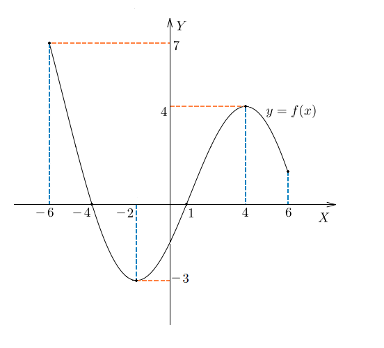
In our figure, the domain of the function is a segment. It is on this segment that the graph of the function is drawn. Only here this function exists.

Function range is the set of values ​​that the variable takes. In our figure, this is a segment - from the lowest to the highest value.

Function zeros- points where the value of the function is equal to zero, i.e. . In our figure, these are the points and .

Function values ​​are positive where . In our figure, these are the intervals and .
Function values ​​are negative where . We have this interval (or interval) from to.

The most important concepts - increasing and decreasing function on some set. As a set, you can take a segment, an interval, a union of intervals, or the entire number line.

Function increases

In other words, the more , the more , that is, the graph goes to the right and up.

Function decreases on the set if for any and belonging to the set the inequality implies the inequality .

For a decreasing function, a larger value corresponds to a smaller value. The graph goes right and down.

In our figure, the function increases on the interval and decreases on the intervals and .

Let's define what is maximum and minimum points of the function.

Maximum point- this is an internal point of the domain of definition, such that the value of the function in it is greater than in all points sufficiently close to it.
In other words, the maximum point is such a point, the value of the function at which more than in neighboring ones. This is a local "hill" on the chart.

In our figure - the maximum point.

Low point- an internal point of the domain of definition, such that the value of the function in it is less than in all points sufficiently close to it.
That is, the minimum point is such that the value of the function in it is less than in neighboring ones. On the graph, this is a local “hole”.

In our figure - the minimum point.

The point is the boundary. It is not an interior point of the domain of definition and therefore does not fit the definition of a maximum point. After all, she has no neighbors on the left. In the same way, there can be no minimum point on our chart.

The maximum and minimum points are collectively called extremum points of the function. In our case, this is and .

But what if you need to find, for example, function minimum on the cut? In this case, the answer is: because function minimum is its value at the minimum point.

Similarly, the maximum of our function is . It is reached at the point .

We can say that the extrema of the function are equal to and .

Sometimes in tasks you need to find the largest and smallest values ​​of the function on a given segment. They do not necessarily coincide with extremes.

In our case smallest function value on the interval is equal to and coincides with the minimum of the function. But its largest value on this segment is equal to . It is reached at the left end of the segment.

In any case, the largest and smallest values ​​of a continuous function on a segment are achieved either at the extremum points or at the ends of the segment.