A very convenient invention of the computer world is spreadsheets. You can enter data into them and beautifully arrange them in the form of documents to your taste (or to the taste of your superiors).
You can create such a document once - in fact, a whole family of documents at once, which in Excel terminology is called a “workbook” ( English version workbook).
How Excel behaves
Then you just need to change a few initial numbers when the data changes, and then Excel will perform several operations at once, arithmetic and others. It's in the document:

To do this, a spreadsheet program (and Excel is far from the only one) has a whole arsenal of arithmetic tools and ready-made functions performed using already debugged and workable programs. You just need to indicate in any cell when writing a formula, among other operands, the name of the corresponding function and the arguments in parentheses to it.
There are a lot of functions and they are grouped by application areas:

There is a whole set of statistical functions for summarizing multiple data. Getting the average value of some data is probably the very first thing that comes to a statistician’s mind when he looks at the numbers.
What is the average?
This is when a certain series of numbers is taken, two values are calculated from them - the total number of numbers and their total sum, and then the second is divided by the first. Then you get a number whose value is somewhere in the very middle of the series. Perhaps it will even coincide with some of the numbers in the series.
Well, let’s assume that that number was terribly lucky in this case, but usually the arithmetic mean not only does not coincide with any of the numbers in its series, but even, as they say, “doesn’t fit into any gates” in this series . For example, average number of people There may be 5,216 people living in apartments in some city in N-Ska. How is that? Are there 5 people living and an additional 216 thousandths of one of them? Those who know will only grin: what are you talking about! These are statistics!
Statistical (or simply accounting) tables can be completely different forms and sizes. Actually, the shape is a rectangle, but they can be wide, narrow, repeating (say, data for a week by day), scattered on different sheets Your workbook - a workbook.
And even in other workbooks (that is, in books, in English), and even on other computers in local network, or, scary to say, in other ends of our white light, now united by the all-powerful Internet. A lot of information can be obtained from very reputable sources on the Internet already in finished form. Then process, analyze, draw conclusions, write articles, dissertations...
As a matter of fact, today we just need to calculate the average on some array of homogeneous data, using the miraculous spreadsheet program. Homogeneous means data about some similar objects and in the same units of measurement. So that people will never be summed up with sacks of potatoes, and kilobytes with rubles and kopecks.
Example of finding the average value
 Let us have the initial data written in some cells. Usually, generalized data, or data obtained from the original data, is somehow recorded here.
The initial data is located on the left side of the table (for example, one column is the number of parts produced by one employee A, which corresponds to a separate line in the table, and the second column is the price of one part), the last column indicates the output of employee A in money.
Previously, this was done using a calculator, now you can do this simple task trust a program that never makes mistakes.
Simple daily earnings table
 Here in the picture amount of earnings and it is calculated for each employee in column E using the formula of multiplying the number of parts (column C) by the price of parts (column D).
Then he won’t even be able to step into other places in the table, and he won’t be able to look at the formulas. Although, of course, everyone in that workshop knows how to produce individual employee goes into the money he earned in a day.
Total values
Then the total values are usually calculated. These are summary figures throughout the workshop, area, or the entire team. Usually these figures are reported by some bosses to others - higher up bosses.
This is how you can calculate the amounts in the source data columns, and at the same time in the derived column, that is, the earnings column
Let me immediately note that while the Excel table is being created, no protection is done in the cells. Otherwise, how would we draw the sign itself, introduce the design, color it and enter smart and correct formulas? Well, when everything is ready, before giving this workbook (that is, a spreadsheet file) to a completely different person, protection is done. Yes, simply from a careless action, so as not to accidentally damage the formula.
And now the self-calculating table will begin to work in the workshop along with the rest of the workshop workers. After the working day is over, all such tables of data about the work of the workshop (and not only one of it) are transferred to high management, who will summarize this data the next day and draw some conclusions.
Here it is, average (mean - in English)
 It comes first will calculate the average number of parts, produced per worker per day, as well as average earnings per day for the workshop workers (and then for the plant). We will also do this in the last, lowest row of our table.
As you can see, you can use the amounts already calculated in the previous line, simply divide them by the number of employees - 6 in this case.
In formulas, divide by constants, constant numbers, This bad taste. What if something out of the ordinary happens to us, and the number of employees becomes smaller? Then you will need to go through all the formulas and change the number seven to some other one everywhere. You can, for example, “deceive” the sign like this:
Instead of a specific number, put in the formula a link to cell A7, where it is serial number the last employee on the list. That is, this will be the number of employees, which means we correctly divide the amount for the column of interest to us by the number and get the average value. As you can see, the average number of parts turned out to be 73 and plus a mind-blowing in terms of numbers (though not in significance) makeweight, which is usually thrown out by rounding.
Rounding to the nearest kopeck
 Rounding is a common action when in formulas, especially accounting ones, one number is divided by another. Moreover, this is a separate topic in accounting. Accountants have been involved in rounding for a long time and scrupulously: they immediately round every number obtained by division to the nearest kopeck.
Excel is a mathematical program. She is not in awe of a share of a penny - where to put it. Excel simply stores the numbers as is, with all decimal places included. And again and again he will carry out calculations with such numbers. And the final result can be rounded (if we give the command).
Only accounting will say that this is a mistake. Because they round each resulting “crooked” number to whole rubles and kopecks. And the end result usually turns out a little different than that of a program indifferent to money.
But now I'll tell you main secret. Excel can find the average value without us; it has a built-in function for this. She only needs to specify the data range. And then she herself will sum them up, count them, and then she herself will divide the amount by the quantity. And the result will be exactly the same as what we comprehended step by step.
In order to find this function, we go to cell E9, where its result should be placed - the average value in column E, and click on the icon fx, which is to the left of the formula bar.
- A panel called “Function Wizard” will open. This is a multi-step dialogue (Wizard, in English), with the help of which the program helps in constructing complex formulas. And, note that the help has already begun: in the formula bar, the program entered the = sign for us.
- Now we can be calm, the program will guide us through all the difficulties (even in Russian, even in English) and as a result it will be built correct formula for calculation.
 In the top window (“Search for function:”) it is written that we can search and find here. That is, here you can write “average” and click the “Find” button (Find, in English). But you can do it differently. We know that this function is from the statistical category. So we will find this category in the second window. And in the list that opens below, we will find the “AVERAGE” function.
At the same time we will see how great it is there many functions in the statistical category, there are 7 averages alone. And for each of the functions, if you move the pointer over them, below you can see a brief summary of this function. And if you click even lower, on the inscription “Help for this function,” you can get a very detailed description of it.
Now we'll just calculate the average. Click “OK” (this is how agreement is expressed in English, although it is more likely in American) on the button below.
The program has entered the beginning of the formula, now you need to set the range for the first argument. Just select it with the mouse. Click OK and get the result. Left add rounding here, which we made in cell C9, and the plate is ready for daily use.
How to calculate the average of numbers in Excel
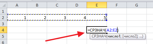
You can find the arithmetic mean of numbers in Excel using the function.
Syntax AVERAGE
=AVERAGE(number1,[number2],…) - Russian version
Arguments AVERAGE
- number1– the first number or range of numbers for calculating the arithmetic mean;
- number2(Optional) – the second number or range of numbers for calculating the arithmetic mean. Maximum amount function arguments – 255.
To calculate, follow these steps:
- Select any cell;
- Write the formula in it =AVERAGE(
- Select the range of cells for which you want to make a calculation;
- Press the “Enter” key on your keyboard
The function will calculate the average value in the specified range among those cells that contain numbers.
How to find the average given text
If there are empty lines or text in the data range, the function treats them as “zero”. If among the data there are logical expressions FALSE or TRUE, then the function perceives FALSE as “zero”, and TRUE as “1”.
How to find the arithmetic mean by condition
To calculate the average by condition or criterion, use the function. For example, imagine that we have data on product sales:

Our task is to calculate the average value of pen sales. To do this, we will take the following steps:
- In cell A13 write the name of the product “Pens”;
- In cell B13 let's introduce the formula:
=AVERAGEIF(A2:A10,A13,B2:B10)
Cell range “ A2:A10” indicates a list of products in which we will search for the word “Pens”. Argument A13 this is a link to a cell with text that we will search among the entire list of products. Cell range “ B2:B10” is a range with product sales data, among which the function will find “Handles” and calculate the average value.

The most common type of average is the arithmetic mean.
Simple arithmetic mean
A simple arithmetic mean is the average term, in determining which the total volume of this characteristic in the data is distributed equally among all units included in the given population. Thus, the average annual output per employee is the amount of output that would be produced by each employee if the entire volume of output were equally distributed among all employees of the organization. The arithmetic mean simple value is calculated using the formula:
Example 1 .Simple arithmetic average— Equal to the ratio of the sum of individual values of a characteristic to the number of characteristics in the aggregate
A team of 6 workers receives 3 3.2 3.3 3.5 3.8 3.1 thousand rubles per month.
Find average salary
Solution: (3 + 3.2 + 3.3 +3.5 + 3.8 + 3.1) / 6 = 3.32 thousand rubles.
Arithmetic average weighted If the volume of the data set is large and represents a distribution series, then the weighted arithmetic mean is calculated. This is how the weighted average price per unit of production is determined: total cost
products (the sum of the products of its quantity and the price of a unit of production) is divided by the total quantity of products.
![]()
— equal to the ratio of (the sum of the products of the value of a feature to the frequency of repetition of this feature) to (the sum of the frequencies of all features). It is used when variants of the population under study occur an unequal number of times. Example 2Let's imagine this in the form of the following formula: Weighted arithmetic average
. Find the average salary of workshop workers per month The average salary can be obtained by dividing total amount wages on

total number
workers:
Answer: 3.35 thousand rubles. Arithmetic mean for interval series When calculating the arithmetic mean for an interval variation series, first determine the mean for each interval as the half-sum of the upper and
lower limits
, and then - the average of the entire series. In the case of open intervals, the value of the lower or upper interval is determined by the size of the intervals adjacent to them. Averages calculated from interval series are approximate. Example 3. Define

average age
evening students. Averages calculated from interval series are approximate. The degree of their approximation depends on the extent to which the actual distribution of population units within the interval approaches uniform distribution. When calculating averages, not only absolute, but also
relative values
(frequency):
![]()
The arithmetic mean has a number of properties that more fully reveal its essence and simplify calculations: 1. The product of the average by the sum of frequencies is always equal to the sum of the products of the variant by frequencies, i.e. 2.Medium
arithmetic sum
![]()
varying quantities is equal to the sum of the arithmetic averages of these quantities:
When working with tables in Excel, you often need to calculate the sum or average. We have already talked about how to calculate the amount.
How to calculate the average of a column, row, or individual cells
The easiest way is to calculate the average of a column or row. To do this, you first need to select a series of numbers that are placed in a column or row. After the numbers are selected, you need to use the “Auto Sum” button, which is located on the “Home” tab. Click on the arrow to the right of this button and select the “Medium” option from the menu that appears.
As a result, their average value will appear next to the numbers. If you look at the line for formulas, it becomes clear that to obtain the average value in Excel, the AVERAGE function is used. You can use this function anywhere convenient place and without the “Auto sum” button.

If you need the average value to appear in some other cell, then you can transfer the result simply by cutting it (CTRL-X) and then pasting (CTRL-V). Or you can first select the cell where the result should be located, and then click on the “Auto Sum - Average” button and select a series of numbers.
If you need to calculate the average value of some individual or specific cells, then this can also be done using the “Auto sum – Average” button. In this case, you must first select the cell in which the result will be located, then click “Auto sum - Average” and select the cells for which you want to calculate the average value. To select individual cells, you need to hold down the CTRL key on your keyboard.

In addition, you can enter a formula to calculate the average of certain cells manually. To do this, you need to place the cursor where the result should be, and then enter the formula in the format: = AVERAGE (D3; D5; D7). Where instead of D3, D5 and D7 you need to indicate the addresses of the data cells you need.
It should be noted that when entering a formula manually, cell addresses are entered separated by commas, and after the last cell there is no comma. After entering the entire formula, you need to press the Enter key to save the result.
How to quickly calculate and view the average in Excel
In addition to everything described above, Excel has the ability to quickly calculate and view the average value of any data. To do this, you just need to select the required cells and look in the lower right corner of the program window.

The average value of the selected cells will be indicated there, as well as their number and sum.
This spreadsheet processor can handle almost all calculations. It is ideal for accounting. There are special tools for calculations - formulas. They can be applied to a range or to individual cells. To find out the minimum or maximum number in a group of cells, you don’t have to look for them yourself. It is better to use the options provided for this. It will also be useful to understand how to calculate the average in Excel.
This is especially true in tables with a large amount of data. If the column, for example, contains product prices shopping center. And you need to find out which product is the cheapest. If you search for it manually, it will take a lot of time. But in Excel this can be done in just a few clicks. The utility also calculates the arithmetic mean. After all, these are two simple operations: addition and division.
Maximum and minimum
Here's how to find maximum value in Excel:
- Place the cell cursor anywhere.
- Go to the "Formulas" menu.
- Click Insert Function.
- Select "MAX" from the list. Or write this word in the "Search" field and click "Find".
- In the "Arguments" window, enter the addresses of the range whose maximum value you need to know. In Excel, cell names consist of a letter and a number (“B1”, “F15”, “W34”). And the name of the range is the first and last cells that are included in it.
- Instead of an address, you can write several numbers. Then the system will show the largest of them.
- Click OK. The result will appear in the cell in which the cursor was located.

Next step - specify the range of values
Now it will be easier to figure out how to find the minimum value in Excel. The algorithm of actions is completely identical. Just replace "MAX" with "MIN".
Average
The arithmetic mean is calculated as follows: add up all the numbers from the set and divide by their number. In Excel, you can calculate amounts, find out how many cells are in a row, and so on. But it's too difficult and time-consuming. You'll have to use a lot different functions. Keep information in your head. Or even write something down on a piece of paper. But the algorithm can be simplified.
Here's how to find the average in Excel:
- Place the cell cursor in any free space in the table.
- Go to the Formulas tab.
- Click on "Insert Function".
- Select AVERAGE.
- If this item is not in the list, open it using the “Find” option.
- In the Number1 area, enter the range address. Or write several numbers in different fields “Number2”, “Number3”.
- Click OK. The required value will appear in the cell.

This way you can carry out calculations not only with positions in the table, but also with arbitrary sets. Excel essentially plays the role of an advanced calculator.
other methods
The maximum, minimum and average can be found in other ways.
- Find the function bar labeled "Fx". It is above the main work area of the table.
- Place the cursor in any cell.
- Enter an argument in the "Fx" field. It starts with an equal sign. Then comes the formula and the address of the range/cell.
- You should get something like “=MAX(B8:B11)” (maximum), “=MIN(F7:V11)” (minimum), “=AVERAGE(D14:W15)” (average).
- Click on the check mark next to the functions field. Or just press Enter. The desired value will appear in the selected cell.
- The formula can be copied directly into the cell itself. The effect will be the same.

The Excel AutoFunctions tool will help you find and calculate.
- Place the cursor in a cell.
- Find a button whose name begins with "Auto". This depends on the default option selected in Excel (AutoSum, AutoNumber, AutoOffset, AutoIndex).
- Click on the black arrow below it.
- Select MIN (minimum value), MAX (maximum), or AVERAGE (average).
- The formula will appear in the marked cell. Click on any other cell - it will be added to the function. “Stretch” the box around it to cover the range. Or click on the grid while holding down the Ctrl key to select one element at a time.
- When finished, press Enter. The result will be displayed in the cell.
In Excel, calculating the average is quite easy. There is no need to add and then divide the amount. There is a separate function for this. You can also find the minimum and maximum in a set. This is much easier than counting by hand or looking for numbers in a huge table. Therefore, Excel is popular in many areas of activity where accuracy is required: business, auditing, human resources, finance, trade, mathematics, physics, astronomy, economics, science.


